GMT Part 3: Working with NetCDF data by creating a synoptic weather map
For my thesis I had to examine synoptic scale circulation over South-Africa, I wanted to recreate a classic synoptic map that represented mean sea level pressure and also geopotentail at 500hPa. I knew the South-African Weather Service (SAWS) has daily maps they make publicly available, but the maps are not always the highest quality as they are hand drawn - a tedious process I would imagine.
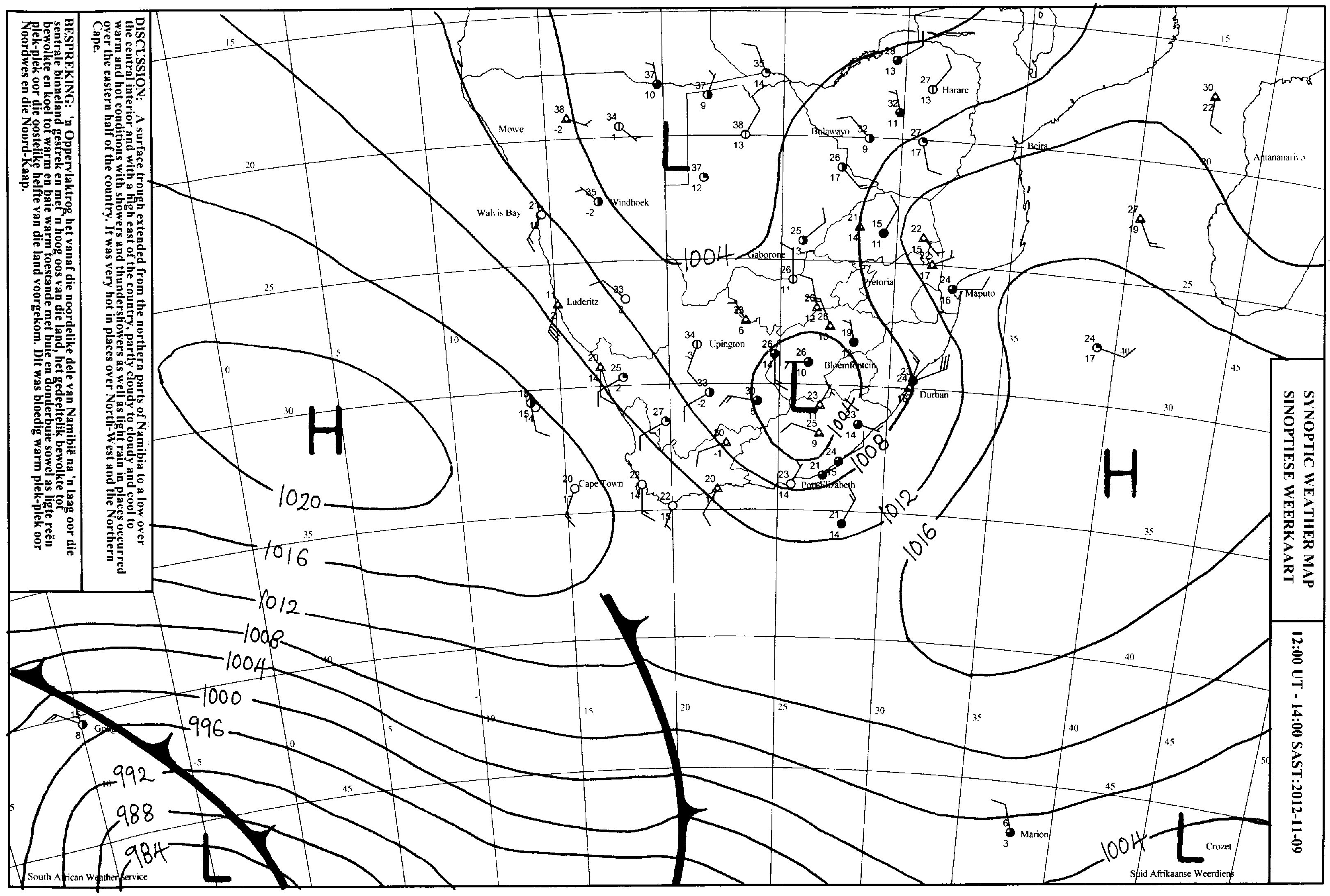 A SAWS synoptic map.
In addition to this I was also attempting to better understand GMT’s handling of NetCDF files. I used ERA-Interim data in my thesis for WRF and also some objective clustering, the ERA dataset was thus the obvious choice. Using GMT to recreate these synoptic maps took me a couple of days, mostly the time consumption was related to handling the NetCDF data. GMT uses Reverse Polish Notation (RPN) for math functions which I needed to figure out as you’ll see. It is also useful to have CDO, ncview and ncdump installed for data inspection and manipulating. A last point is that I compiled it all in a bash script, this is useful for various reasons, so just learn to do it.
First off a synoptic map is pretty simple, it consists of pressure levels and if you really want you can add some other variables such as CAPE, temperature, precipitate water, and so forth. Synoptic mainly refers to a scale in this context if you wondered, a 1975 paper by Isidoro Orlanski explains this concept of scale related to weather and climate clearly. You’ll notice is that the projection used in the SAWS map is not the Mercator projection I’ve used previously, but instead a equal area projection, namely Lambert Azimuthal Equal-Area. Coincidently someone already explained the projection using South-Africa as an example.
A quick drawing of the basemap and we can see th projection is similar,
gmt psbasemap -R-20/-46/60/-12r -JA25/-30/25.5 -Xc -Yc -B15a0g15 -K > lambert_base.ps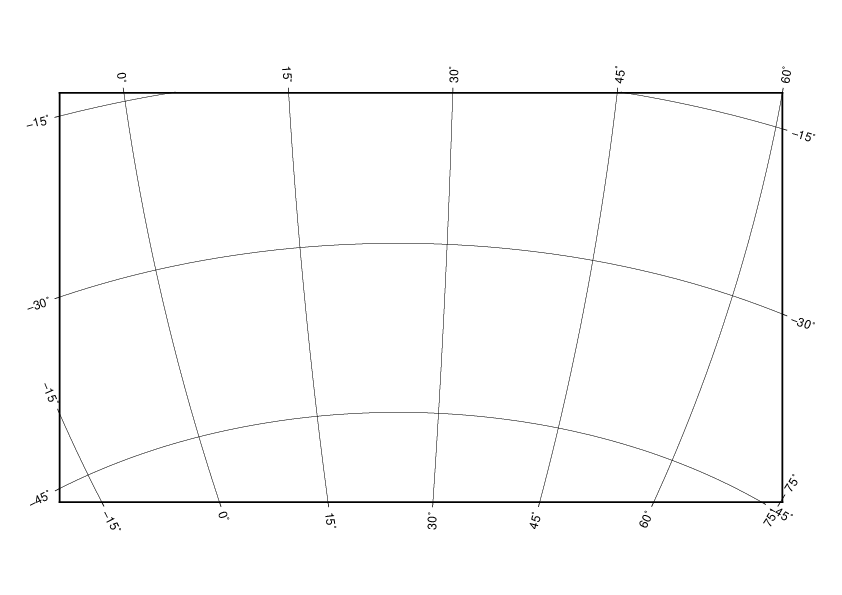
This does not mean a lot without any land referance, the -K option tells us we want to add something later to the map. Using pscoast and -Df and -N1 options we can add coastlines and national borders to this map,
gmt pscoast -R -JA -W -Df -N1 -O -K >> lambert_base.ps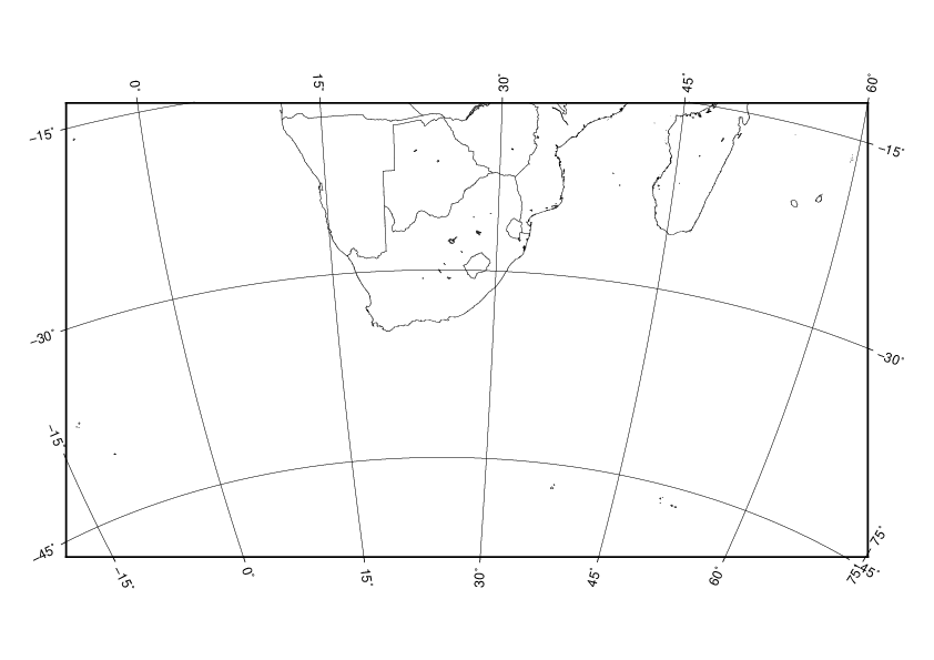
That was pretty straight forward, we can see that the map is more or less similar to the synoptic map we want to make. Now we need to add the pressure lines to the map, this gets a little more tricky. As mentioned, I used ERA-Interim data in my thesis, the data is maintained by the ECMWF and publicly available, you do however need to sign up to use the data. You can download the data directly from the website, it is however easier to use the ECMWF Python API. Do this to use the script I wrote below, otherwise it will not work and you’ll think I’m stupid. So, once you’ve got that set up the rest will make a little more sense.
I initially tried to just run gmt grdimage without any data conversion, this did not work. Inspecting the ordinal data with,
ncdump -h msl.nc Shows us the msl variable is is present,
netcdf msl {
dimensions:
	longitude = 480 ;
	latitude = 241 ;
	time = UNLIMITED ; // (1 currently)
variables:
	float longitude(longitude) ;
		longitude:units = "degrees_east" ;
		longitude:long_name = "longitude" ;
	float latitude(latitude) ;
		latitude:units = "degrees_north" ;
		latitude:long_name = "latitude" ;
	int time(time) ;
		time:units = "hours since 1900-01-01 00:00:0.0" ;
		time:long_name = "time" ;
		time:calendar = "gregorian" ;
	short msl(time, latitude, longitude) ;
		msl:scale_factor = 0.130510582454641 ;
		msl:add_offset = 99611.2472447088 ;
		msl:_FillValue = -32767s ;
		msl:missing_value = -32767s ;
		msl:units = "Pa" ;
		msl:long_name = "Mean sea level pressure" ;
		msl:standard_name = "air_pressure_at_sea_level" ;
I think the data needs to be in a 2-dimensional grid, explained here in more detail. To get a GMT compliant file we need to do,
gmt grdconvert 'msl.nc?msl' -Gmslp_org.ncInspecting the data shows us that z has replaced msl
netcdf mslp_org {
dimensions:
	lon = 480 ;
	lat = 241 ;
variables:
	double lon(lon) ;
		lon:long_name = "longitude" ;
		lon:units = "degrees_east" ;
		lon:actual_range = -180., 179.25 ;
	double lat(lat) ;
		lat:long_name = "latitude" ;
		lat:units = "degrees_north" ;
		lat:actual_range = -90., 90. ;
	float z(lat, lon) ;
		z:long_name = "Mean sea level pressure" ;
		z:units = "Pa" ;
		z:_FillValue = NaNf ;
		z:actual_range = 95334.9375, 103887.6875 ;
We can also see that 95334 is not a pressure value, we have to divide it by 100. It is possible to use CDO or NCO tools, but the powerful GMT has math functions in the form of Reverse Polish Notation (RPN). To convert new mslp value by a 100 we can do
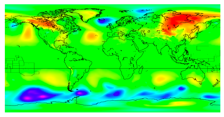
gmt grdmath mslp_org.nc 100 DIV = mslp_nrm.ncBecause the data covers the whole word we can make a quick plot without to much trouble using grdimage to see if everything seems realistic enough.
gmt grdimage mslp_nrm.nc -JX25/0d -K > mslp.ps
gmt pscoast -Rmslp_nrm.nc -JX -W0.5 -N3 -O -Dc >> mslp.ps
This gives us a image of the mslp scaled and covering the whole world.
We do however want a contoured mslp and also clip it to South-Africa. To do this we need to call the psbasemap and pscoast functions we used earlier and then use grdcontour to contour the data.
gmt psbasemap -R-20/-46/60/-12r -JA25/-30/25.5 -Xc -Yc -B15a0g15 -K > synoptic_map.ps
gmt pscoast -R -JA -W -Df -N1 -O -K >> synoptic_map.ps
gmt grdcontour -R -JA -Wthinnest mslp_nrm.nc -C4 -A4 -O -K >> synoptic_map.ps
We get a nice map with the MSLP contoured over South-Africa, much like
the original synoptic map.
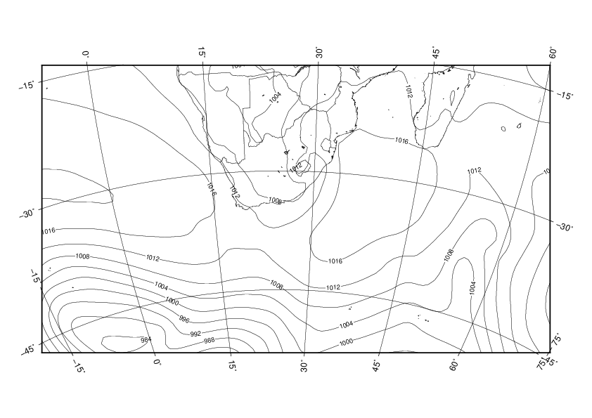
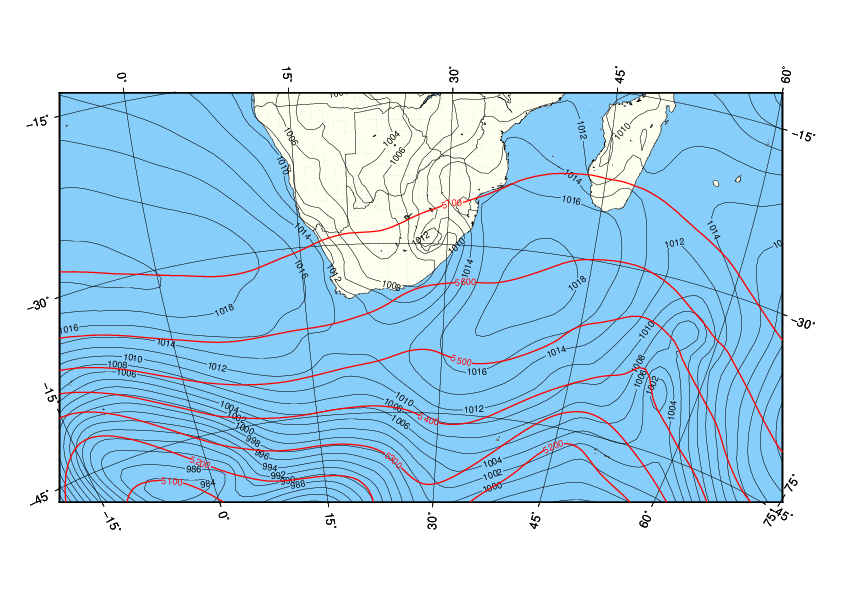
We can see that the ERA created map captures similar features as the SAWS synoptic map; note the South-Indian Ocean High Pressure and the South-Atlantic High Pressure and the low pressure from the Easterly Wave over the Country. To add the L and H indicators I would use inkscape at this time, a script would be possible but that is beyond me right now. The weather stations indicators would also theoretically be possible and I’ll try to figure that out in the future. The below map is the final map I created, you can see The script below does all the above steps with the addition of the upper 500hPa geopotential. I also added some color. In the end we end up with a new and improved (in my subjective opinion) synoptic map as seen below.
#!/bin/bash

####################################################
# This is to make a synotpic map                   #
# See below source for some more info              #
# http://gmt.soest.hawaii.edu/boards/1/topics/5997 #
####################################################

####################################################
# Step 1: Download the ERA-DATA with this script   #
####################################################

python << EOF
from ecmwfapi import ECMWFDataServer
server = ECMWFDataServer()
server.retrieve({
    "class": "ei",
    "dataset": "interim",
    "date": "2012-11-09/to/2012-11-09",
    "expver": "1",
    "grid": "0.75/0.75",
    "levtype": "sfc",
    "param": "151.128",
    "step": "0",
    "stream": "oper",
    "time": "12:00:00",
    "type": "an",
    "format":"netcdf",
    "target": "msl.nc",
})

server.retrieve({
    "class": "ei",
    "dataset": "interim",
    "date": "2012-11-09/to/2012-11-09",
    "expver": "1",
    "grid": "0.75/0.75",
    "levelist": "500",
    "levtype": "pl",
    "param": "129.128",
    "step": "0",
    "stream": "oper",
    "time": "12:00:00",
    "type": "an",
    "format":"netcdf",
    "target": "zg500.nc",
})
EOF

read -p "ERA-Data downloaded. Press enter to continue and convert data for use in GMT "

#############################################################################
# The file is not compatible with GMT, to get it to work do ?msl           #
# selects the variable we want and writes it to mslp.nc. The '' is         #
# important otherwise bash looks for a wildcard.                           #
# The units are also wrong to correct them we need to use gmt grdmath      #
#############################################################################

gmt grdconvert 'msl.nc?msl' -Gmslp_org.nc
gmt grdedit mslp_org.nc -R-180/180/-90/90 -S
gmt grdmath mslp_org.nc 100 DIV = mslp_nrm.nc

gmt grdconvert 'zg500.nc?z' -Gzg500_org.nc
gmt grdedit zg500_org.nc -R-180/180/-90/90 -S
gmt grdmath zg500_org.nc 10 DIV = zg500_nrm.nc

read -p "Lets inspect the data with ncdump. Press enter to continue "
ncdump -h mslp_nrm.nc
ncdump -h zg500_nrm.nc

read -p "Lets inspect the data with grdinfo. Press enter to continue "
gmt grdinfo mslp_nrm.nc
gmt grdinfo zg500_nrm.nc

####################################################
# Here we create a very basic map to view our data #
####################################################
read -p "Lets create a world map. Press enter to continue "

echo 'MSLP map '
gmt grdimage mslp_nrm.nc -JX25/0d -K > mslp.ps
gmt pscoast -Rmslp_nrm.nc -JX -W0.5 -N3 -O -Dc >> mslp.ps

echo 'Geopotential map '
gmt grdimage zg500_nrm.nc -JX25/0d -K > zg500.ps
gmt pscoast -Rzg500_nrm.nc -JX -W0.5 -N3 -O -Dc >> zg500.ps

read -p "World map created. We will now create a map of South-Africa. Press enter to continue "

#################################################################################
# Now we need to create a contoured map from the netcdf file for SA             #
# See https://www.soest.hawaii.edu/gmt/gmt/html/man/gmtcolors.html              #
# http://gmt.soest.hawaii.edu/doc/latest/GMT_Docs.html#specifying-pen-attributes#
#################################################################################
out=southafrica_syn.ps

#Coordinates (actually lower left and upper right not E S W N)
east=-20
south=-46
west=60
north=-12r

#Projection (Lambert Azimuthal Equal-Area)
width=25.5

gmt psbasemap  -R$east/$south/$west/$north -JA25/-30/$width -Xc -Yc -B15a0g15 -K > $out
gmt pscoast    -R -JA -Df -N1 -W -Givory -B -Slightskyblue -O -K >> $out
gmt grdcontour -R -JA -Wthinnest mslp_nrm.nc -C2 -A2 -O -K >> $out
gmt grdcontour -R -JA -Wthick,red zg500_nrm.nc -C100 -A100+v -P -Gn1 -O -K >> $out

read -p "Done. Press enter to continue "