Shapefiles in R - extracting polygons
This builds on the previous post Shapefiles in R - making a basic map.
In QGIS or ArcGIS is pretty easy to extract part of a shapefile. Generally you can open shapefile attribute table and select the feature you want and delete the rest. In R it’s also pretty easy, but less mouse clicking and more typing kinda easy.
In R do:
library(ggplot2)
library(rgdal)
library(rgeos)
theme_set(theme_classic(base_size=22))
#Define the basemap as basemap, where dsn == the directory where the shapefile
#is located. For ggplot use map_data function:
basemap <- map_data(readOGR(dsn="./", layer="ZAF_adm1"))
#To actually work with the shapefiles, omit the map_data function
#and invoke it later
basemap_1 <- readOGR(dsn="./", layer="ZAF_adm1")
ecoregions <- readOGR(dsn="./", layer="Ecoregions2017")
# To extract a layer to use in a plot, in this case Gauteng and the Highveld,
# do:
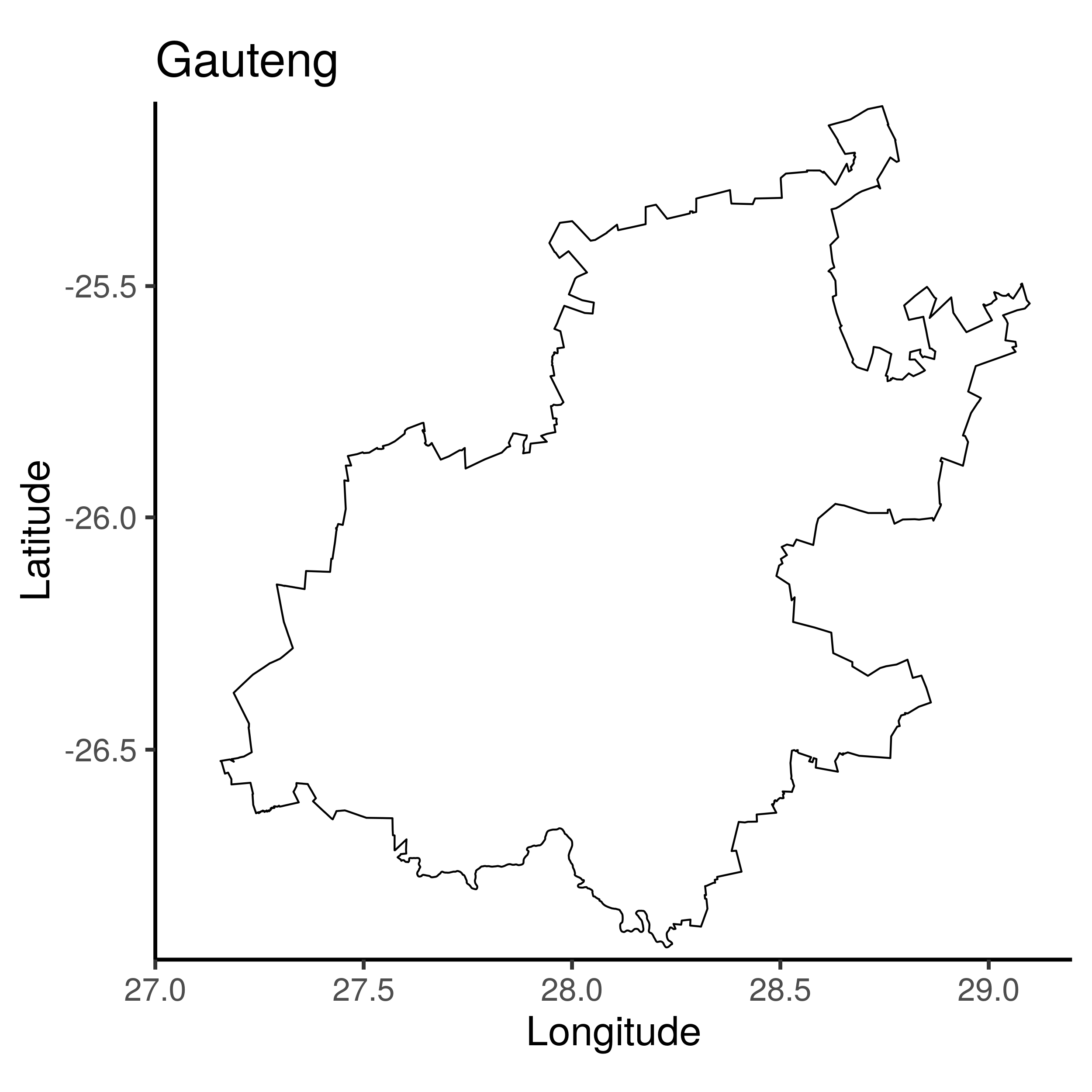
gauteng <- map_data(basemap_1[basemap_1$NAME_1=="Gauteng", ])
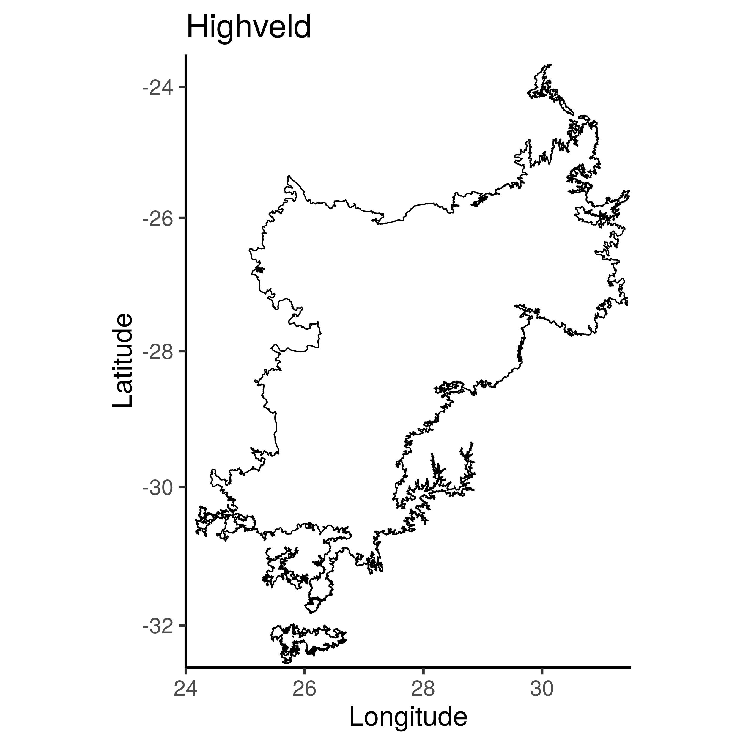
highveld <- map_data(ecoregions[ecoregions$ECO_ID=="81", ])
# Get the map extent for the boundries
summary(highveld)
summary(gauteng)
plt_hv <- ggplot() +
geom_path(data=highveld, aes(x=long, y=lat, group=group)) +
coord_map(ylim=c(-23.5,-32.6), xlim=c(24, 31.5)) +
ggtitle("Highveld") +
ylab("Latitude") + xlab("Longitude")
plt_gp <- ggplot() +
geom_path(data=gauteng, aes(x=long, y=lat, group=group)) +
coord_map(ylim=c(-25.1,-26.95), xlim=c(27, 29.2)) +
ggtitle("Gauteng") +
ylab("Latitude") + xlab("Longitude")
#To see the map
plt_gp
plt_highveld
#To see the map
png("Highveld.png", width = 6 * 500, height = 5 * 500, res = 300)
plt_hv
dev.off()
png("Gauteng.png", width = 5 * 500, height = 5 * 500, res = 300)
plt_gp
dev.off()The maps: